Linear Regression with Regularization

Regularization is a way to prevent overfitting and allows the model to generalize better. We’ll cover the Ridge and Lasso regression here.

The Need for Regularization

Unlike polynomial fitting, it’s hard to imagine how linear regression can overfit the data, since it’s just a single line (or a hyperplane). One situation is that features are correlated or redundant.

Suppose there are two features, both are exactly the same, our predicted hyperplane will be in this format:

\[\hat{y} = w_0 + w_1x_1 + w_2x_2\]

and the true values of \(x_2\) is almost the same as \(x_1\) (or with some multiplicative factor and noise). Then, it’s best to just drop \(w_2x_2\) term and use:

\[\hat{y} = w_0 + w_1x_1\]

to fit the data. This is a simpler model.

But we don’t know whether \(x_1\) and \(x_2\) is actually redundant or not, at least with bare eyes, and we don’t want to manually drop a parameter just because we feel like it. We want to model to learn to do this itself, that is, to prefer a simpler model that fits the data well enough.

To do this, we add a penalty term to our loss function. Two common penalty terms are L2 and L1 norm of \(w\).

L2 and L1 Penalty

0. No Penalty (or Linear)

This is linear regression without any regularization (from previous article):

\[L(w) = \sum_{i=1}^{n} \left( y^i - wx^i \right)^2\]

1. L2 Penalty (or Ridge)

We can add the L2 penalty term to it, and this is called L2 regularization.:

\[L(w) = \sum_{i=1}^{n} \left( y^i - wx^i \right)^2 + \lambda\sum_{j=0}^{d}w_j^2\]

This is called L2 penalty just because it’s a L2-norm of \(w\). In fancy term, this whole loss function is also known as Ridge regression.

Let’s see what’s going on. Loss function is something we minimize. Any terms that we add to it, we also want it to be minimized (that’s why it’s called penalty term). The above means we want \(w\) that fits the data well (first term), but we also want the values of \(w\) to be small as possible (second term). The lambda (\(\lambda\)) is there to adjust how much to penalize \(w\). Note that sklearn refers to this as alpha (\(\alpha\)) instead, but whatever.

It’s tricky to know the appropriate value for lambda. You just have to try them out, in exponential range (0.01, 0.1, 1, 10, etc), then select the one that has the lowest loss on validation set, or doing k-fold cross validation.

Setting \(\lambda\) to be very low means we don’t penalize the complex model much. Setting it to \(0\) is the original linear regression. Setting it high means we strongly prefer simpler model, at the cost of how well it fits the data.

Closed-form solution of Ridge

It’s not hard to find a closed-form solution for Ridge, first write the loss function in matrix notation:

\[L(w) = {\left\lVert y - Xw \right\rVert}^2 + \lambda{\left\lVert w \right\rVert}_2^2\]

Then the gradient is:

\[\nabla L_w = -2X^T(y-Xw) + 2\lambda w\]

Setting to zero and solve:

\[\begin{split}\begin{align} 0 &= -2X^T(y-Xw) + 2\lambda w \\ &= X^T(y-Xw) - \lambda w \\ &= X^Ty - X^TXw - \lambda w \\ &= X^Ty - (X^TX + \lambda I_d) w \end{align}\end{split}\]

Move that to other side and we get a closed-form solution:

\[\begin{split}\begin{align} (X^TX + \lambda I_d) w &= X^Ty \\ w &= (X^TX + \lambda I_d)^{-1}X^Ty \end{align}\end{split}\]

which is almost the same as linear regression without regularization.

2. L1 Penalty (or Lasso)

As you might guess, you can also use L1-norm for L1 regularization:

\[L(w) = \sum_{i=1}^{n} \left( y^i - wx^i \right)^2 + \lambda\sum_{j=0}^{d}\left|w_j\right|\]

Again, in fancy term, this loss function is also known as Lasso regression. Using matrix notation:

\[L(w) = {\left\lVert y - Xw \right\rVert}^2 + \lambda{\left\lVert w \right\rVert}_1\]

It’s more complex to get a closed-form solution for this, so we’ll leave it here.

Visualizing the Loss Surface with Regularization

Let’s see what these penalty terms mean geometrically.

L2 loss surface

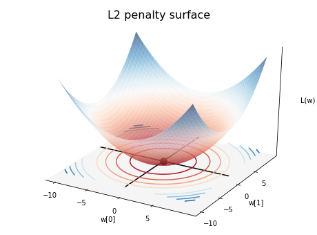
This simply follows the 3D equation:

\[L(w) = {\left\lVert w \right\rVert}_2^2 = w_0^2 + w_1^2\]

The center of the bowl is lowest, since w = [0,0], but that is not even a line and it won’t predict anything useful.

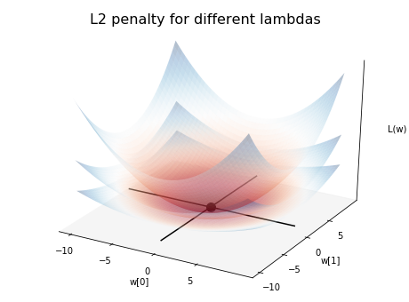
L2 loss surface under different lambdas

When you multiply the L2 norm function with lambda, \(L(w) = \lambda(w_0^2 + w_1^2)\), the width of the bowl changes. The lowest (and flattest) one has lambda of 0.25, which you can see it penalizes The two subsequent ones has lambdas of 0.5 and 1.0.

L1 loss surface

Below is the loss surface of L1 penalty:

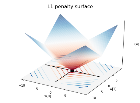
Similarly the equation is \(L(w) = \lambda(\left| w_0 \right| + \left| w_1 \right|)\).

Contour of different penalty terms

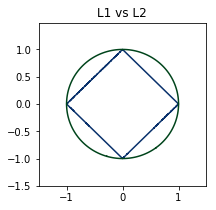
If the L2 norm is 1, you get a unit circle (\(w_0^2 + w_1^2 = 1\)). In the same manner, you get “unit” shapes in other norms:

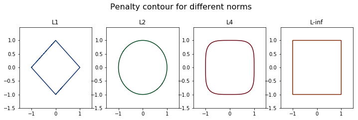
When you walk along these lines, you get the same loss, which is 1

These shapes can hint us different behaviors of each norm, which brings us to the next question.

Which one to use, L1 or L2?

What’s the point of using different penalty terms, as it seems like both try to push down the size of \(w\).

Turns out L1 penalty tends to produce sparse solutions. This means many entries in \(w\) are zeros. This is good if you want the model to be simple and compact. Why is that?

Geometrical Explanation

Note: these figures are generated with unusually high lambda to exaggerate the plot

First let’s bring both linear regression and penalty loss surface together (left), and recall that we want to find the minimum loss when both surfaces are summed up (right):

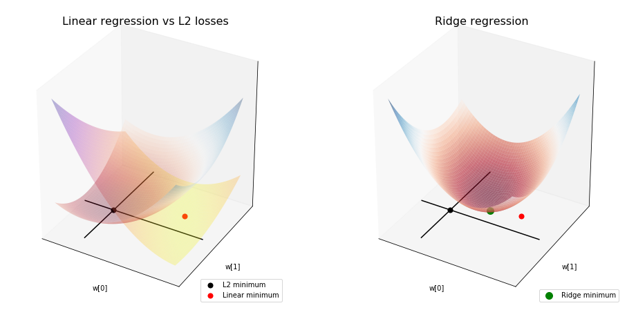
Ridge regression is like finding the middle point where the loss of a sum between linear regression and L2 penalty loss is lowest:

You can imagine starting with the linear regression solution (red point) where the loss is the lowest, then you move towards the origin (blue point), where the penalty loss is lowest. The more lambda you set, the more you’ll be drawn towards the origin, since you penalize the values of :math:`w_i` more so it wants to get to where they’re all zeros:

Since the loss surfaces of linear regression and L2 norm are both ellipsoid, the solution found for Ridge regression tends to be directly between both solutions. Notice how the summed ellipsoid is still right in the middle.

---

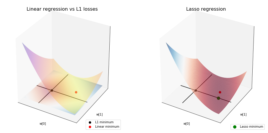
For Lasso:

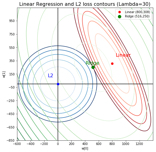
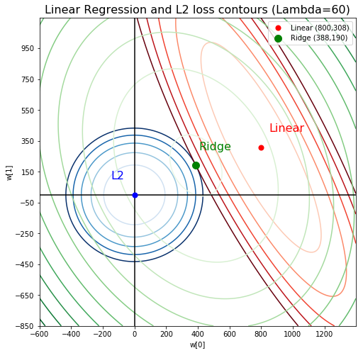
And this is the Lasso solution for lambda = 30 and 60:

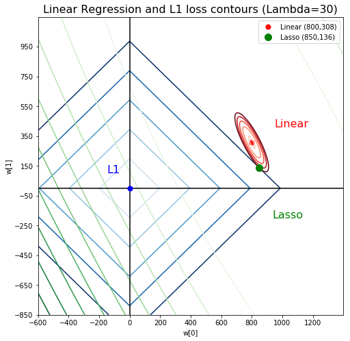
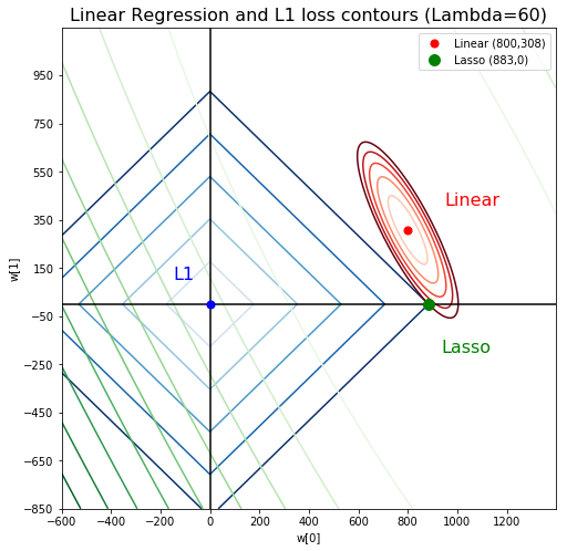
Notice that the ellipsoid of linear regression approaches, and finally hits a corner of L1 loss, and will always stay at that corner. What does a corner of L1 norm means in this situation? It means \(w_1 = 0\).

Again, this is because the contour lines at the same loss value of L2 norm reaches out much farther than L1 norm:

If the linear regression finds an optimal contact point along the L2 circle, then it will stop since there’s no use to move sideways where the loss is usually higher. However, with L1 penalty, it can drift toward a corner, because it’s the same loss along the line anyway (I mean, why not?) and thus is exploited, if the opportunity arises.